

Blog Post | On the Depth of Penetration
Last updated 10/11/2018
Collision physics in Virtual CRASH is based on rigid body dynamics. In particular, most vehicle versus vehicle impacts in Virtual CRASH are simulated using the Kudlich-Slibar impulse-momentum model. This model dates back to the 1960s [1, 2] and is the basis for other vehicle collision simulators used for accident reconstruction [3, 4]. Impulse-momentum simulators are based on Newton’s Laws. Newton’s 3rd Law in particular, of course, leads to momentum conservation. Note, similar impulse-momentum calculations are commonly performed by accident reconstructionists, often by hand, or using other standard calculation applications [5]. The benefit of calculations based on conservation laws of physics is that they bypass the need to model the specific details of how collision forces dynamically evolve, which reduces the problem of predicting collision outcomes to a problem of accounting for known conserved quantities – namely, momentum and energy. For example, arriving at a reasonable estimate of an in-line impact \(\Delta v\) for a target vehicle known to be initially at rest only requires knowledge of the bullet vehicle’s pre-impact speed, vehicle weights, and coefficient of restitution, but does not require knowing whether the impact occurred over a 120 millisecond or 200 millisecond duration, nor does it require detailed knowledge of either vehicle’s force response as a function of crush damage.

Impulse-momentum collision models differ from SMAC-based models [6]. SMAC-based models, which are one type of a general class of simulated contact models referred to as “penalty methods,” typically treat vehicles as though they are composed of ensembles of linear springs which undergo dynamic force balancing at each time step, whose net result is to impart the sum over all springs' resulting forces onto the whole of the parent vehicle. The force on each vehicle evolves, therefore, incrementally over many time-steps until the surfaces of contact are no longer interpenetrating or some other termination condition is satisfied. In rigid body dynamics models, the interacting vehicles exchange discrete impulses at single instants in time, and these impulses are intended to characterize the net effect of all interactions between the vehicles at once, by taking advantage of conservation laws which must be satisfied, to a good approximation, in motor vehicle collisions. Ultimately, both approaches aim to accomplish the same task, which is to prevent ongoing simulated intervehicle penetration by modifying the linear and angular velocities of the colliding vehicles in a manner consistent with the laws of physics.
In the case of impulse-momentum based models, like Virtual CRASH, collapsing all force information into a single exchange of impulses at a single moment in time is analogous to what is done in CRASH3 [7] calculations where, in the case of non-central impacts, one must obtain force centroids based on crush damage patterns, and from these, estimate appropriate lever-arms based on these points to the centers-of-gravity. From these, the “effective mass” for each vehicle can be obtained [8].

To account for the effect of crushing material, Virtual CRASH places the impulse centroid position within the volumes of each vehicle (see figure below).

The distance between the impulse centroid location to the undamaged vehicle mesh is determined in part by the “depth of penetration” parameter [9]. The depth of penetration parameter determines the amount of time the 3D vehicle meshes pass through each other before allowing the impulses to be exchanged. In Virtual CRASH, this value is set to 30 milliseconds by default. That is, starting from the moment the vehicles first overlap, an impulse will be applied 30 milliseconds later. The impulse centroid’s x-y position will be automatically placed near the geometrical center of the overlapping x-y projected area of the vehicles (approximately the mid-point of the crush volume as viewed from above projected onto the x-y plane). The depth of penetration value is adjustable (in the defaults menu of the corresponding ees object), which allows users to have direct control over the total crush damage across the interacting vehicles.
To understand the origin of the 30 milliseconds default depth of penetration value, it is first useful to consider the behavior of a 1-D collision model between two mass-spring objects. Such simplified linear force models have been a standard way to model vehicle impacts for many decades. Below, we present a derivation of the depth of penetration parameter, and its reasonable range of values, based on the expected behavior of a linear spring model. This derivation can also be found in the CRASH3 manual [10].
The 1-D Simple Harmonic Oscillator Model
Suppose we have a spring with spring stiffness given by \(k_{1}\) attached to a block with mass \(m_{1}\) (see figure below).
FIgure adapted from reference [7].
This is made to collide with another mass-spring with stiffness \(k_{2}\) and mass \(m_{2}\). Let us call the position of block 1’s center-of-gravity \(x_{1}(t)\) and block 2’s center-of-gravity \(x_{2}(t)\). Again, these are constrained to move along a single dimension (the \(\hat{x}\)-axis). The point-of-contact between springs (point of contact) is given by point \(x’(t)\), which itself may move as a function of time. Let us define the distance between block 1’s center-of-gravity and the point-of-contact by:
$$ D_{1}(t) = x’(t) – x_{1}(t) \tag{1} $$
For block 2, we have:
$$ D_{2}(t) = x_{2}(t) – x’(t) \tag{2} $$
At \(t = 0\), our initial distances are given by:
$$ D_{1,i} = x’(0) – x_{1}(0) \tag{3} $$
For block 2, we have:
$$ D_{2,i} = x_{2}(0) – x’(0) \tag{4} $$
which are simply the distances between centers-of-gravity and the initial points of contact on each vehicle. For example, for a collinear front-to-rear impact, these might represent the distances between the vehicle centers-of-gravity to outermost surface of the bumpers.
Next, we can define the amount of compression (crush damage) each spring undergoes as a function of time. This is given by:
$$C_{1}(t) = D_{1,i} – D_{1}(t) \tag{5} $$
and
$$C_{2}(t) = D_{2,i} – D_{2}(t) \tag{6}$$
Using equations (5) and (6), the total compression can then be written as:
$$ C_{T}(t) = C_{1}(t) + C_{2}(t) $$
$$ = (D_{1,i} – D_{1}(t)) + (D_{2,i} – D_{2}(t)) $$
$$ = (D_{1,i} – x’(t) + x_{1}(t)) + (D_{2,i} - x_{2}(t) + x’(t)) $$
which simplifies to:
$$ C_{T}(t) = (D_{1,i} + D_{2,i} ) - (x_{2}(t) – x_{1}(t)) \tag{7}$$
Taking the first derivative with respect to time of equation (7) yields (using dot notation):
$$ \dot{C}_{T}(t) = -(\dot{x}_{2}(t) - \dot{x}_{1}(t)) = v_{Rel}(t) \tag{8} $$
That is, the time rate of change of the total crush damage is equivalent to the relative velocity, \(v_{Rel}(t)\), between the centers-of-gravity, where the relative velocity function is given by:
$$v_{Rel}(t) = \dot{x}_{1}(t) - \dot{x}_{2}(t) \tag{9} $$
The second time derivative gives:
$$ \ddot{C}_{T}(t) = -(\ddot{x}_{2}(t) - \ddot{x}_{1}(t)) = a_{Rel}(t) \tag{10} $$
which is the acceleration of block 1’s centers-of-gravity relative to block 2.
Note, we have defined our distance functions such that \(C_{1}\) and \(C_{2}\) remain positive in cases where the distance functions are limited to the range:
$$ D_{1}(t) \leq D_{1,i} $$
and
$$ D_{2}(t) \leq D_{2,i} $$
These are appropriate for modeling vehicles undergoing crushing.
From Newton’s 2nd Law and Hooke’s Law [11], we expect the force on block 1 to be given by:
$$F_{1}(t) = m_{1} \ddot{x}_{1}(t) = -k_{1} \cdot C_{1}(t) \tag{11} $$
The force on block 2 is given by:
$$F_{2}(t) = m_{2} \ddot{x}_{2}(t) = k_{2} \cdot C_{2}(t) \tag{12} $$
These forces are related to each other by Newton’s 3rd law:
$$ k_{1} \cdot C_{1}(t)= k_{2} \cdot C_{2}(t) $$
Using equations (1), (2), (5) and (6), we can expand the above to:
$$ k_{1} \cdot (D_{1,i} – (x’(t) – x_{1}(t))) = k_{2} \cdot ((x_{2}(t) – x’(t)) – D_{2,i}) $$
Using this, we can solve for the point-of-contact position \(x’(t)\):
$$x’(t) = {k_{1}D_{1,i} – k_{2}D_{2,i} + k_{1}x_{1}(t) + k_{2}x_{2}(t) \over k_{1} + k_{2}} \tag{13}$$
Using equation (13), we can therefore rewrite \(C_{1}\) by:
$$ C_{1}(t) = D_{1,i} – (x’(t) – x_{1}(t)) $$
$$ = D_{1,i} – \left({k_{1}D_{1,i} – k_{2}D_{2,i} + k_{1}x_{1}(t) + k_{2}x_{2}(t) \over k_{1} + k_{2}} – x_{1}(t)\right) $$
$$ = {1 \over k_{1} + k_{2}}\cdot \left( k_{1}D_{1,i}+k_{2}D_{1,i}– k_{1}D_{1,i} + k_{2}D_{2,i} - k_{1}x_{1}(t) - k_{2}x_{2}(t) + k_{1}x_{1}(t) + k_{2}x_{1}(t) \right) $$
which simplifies to:
$$ C_{1}(t) = {k_{2} \over k_{1} + k_{2}} \cdot \left( (D_{1,i} + D_{2,i}) – (x_{2}(t) – x_{1}(t)) \right) $$
or,
$$ C_{1}(t) = {k_{2} \over k_{1} + k_{2}} \cdot C_{T}(t) \tag{14} $$
Similarly, for \(C_{2}(t)\), we have:
$$ C_{2}(t) = {k_{1} \over k_{1} + k_{2}} \cdot C_{T}(t) \tag{15}$$
Returning to equations (11) and (12), we can write expressions for the accelerations of our centers-of-gravity:
$$ \ddot{x}_{1}(t) = -{k_{1} \over m_{1}}\cdot C_{1}(t) \tag{16}$$
and
$$ \ddot{x}_{2}(t) = {k_{2} \over m_{2}}\cdot C_{2}(t) \tag{17}$$
Subtracting these gives:
$$ \ddot{x}_{2}(t) - \ddot{x}_{1}(t) = -\ddot{C}_{T}(t) = {k_{2} \over m_{2}}\cdot C_{2}(t) + {k_{1} \over m_{1}}\cdot C_{1}(t) $$
$$ = \left( {k_{1}k_{2} \over k_{1} + k_{2}} \right) \cdot \left( {1 \over m_{1}} + {1 \over m_{2}} \right) \cdot C_{T}(t) $$
We arrive at our final result:
$$\ddot{C}_{T}(t) + \omega^2 C_{T} = 0 \tag{18}$$
where,
$$\omega^2 = {k’ \over m’} \tag{19}$$
$$k’ = {k_{1}k_{2}\over k_{1}+k_{2}} \tag{20}$$
and
$$m’ = {m_{1}m_{2} \over m_{1} + m_{2} } \tag{21}$$
Equation (18) is the deferential equation describing a simple harmonic oscillator [11], whose general solution is given by:
$$ C_{T}(t) = A\sin(\omega t) + B\cos(\omega t) \tag{22}$$
The initial condition for total crush of course is zero, thus giving us \(B\):
$$ C_{T}(0) = B = 0$$
This then implies equation (22) becomes:
$$C_{T}(t) = A\sin(\omega t) \tag{23}$$
Taking the first derivative of equation (23) with respect to time, we have:
$$ \dot{C}_{T}(t) = \omega A \cos(\omega t)$$
Our initial condition for \(\dot{C}\) is simply given by:
$$\dot{C}_{T}(0) = \omega A = v_{Rel,i} $$
We therefore have \(A = {v_{Rel,i} \over \omega} \). This gives our solution:
$$ C_{T}(t) = v_{Rel,i} \sqrt{ {m’ \over k’ }} \cdot \sin\left( \sqrt{ {k’ \over m’ }} \cdot t \right) \tag{24}$$
This relationship tells us then that the total crush damaged imparted to our vehicles is determined by the stiffness values, masses, and closing-speed.
Arriving at Depth of Penetration
Using equation (24), we can now solve for the moment in time at which maximum engagement occurs (“maximum crush”). We can do this by finding the solution to:
$$ \dot{C}_{T}(t’) = v_{Rel}(t’) =v_{Rel,i} \cdot \cos\left( \sqrt{ {k’ \over m’ }} \cdot t’ \right) = 0$$
That is, by solving for the moment in time, \(t’\), at which the centers-of-gravity reach common velocity.
This is given by a solution to the condition:
$$\cos(\sqrt{{k’ \over m’}} t’) = 0$$
Whose general solution is:
$$ \sqrt{{k’ \over m’}} t’ = (2n+1){\pi \over 2}$$
where n is any integer for an oscillating system.
In particular, we are only interested in the \(n = 0\) solution. Thus, we have:
$$ \sqrt{{k’ \over m’}} t’ = {\pi \over 2}$$
or
$$t’ = t_{max} = {\pi \over 2} \cdot \sqrt{m’ \over k’} \tag{25} $$
At this instant, \(t’\), the total crush is at its maximum value. Let us call this time, \(t_{max}\). At this time, the maximum total crush is given by:
$$ C(t_{max}) = v_{Rel,i} \cdot \sqrt{m’/k’} = v_{Rel,i} \cdot {2 \over \pi} \cdot t_{max} \tag{26} $$
Let’s now associate an effective crash pulse half-width given by:
$$\Delta t_{p} = {2 \over \pi} \cdot t_{max} \tag{27} $$
That is:
$$\Delta t_{p} = \sqrt{m’ \over k’} \tag{28} $$
where \(\Delta t_{p} \) is the “depth of penetration” time. Equation (28) tells us one can obtain the depth of penetration for a system by simply knowing the reduced mass and effective stiffness.
With this, we now have:
$$ C(t_{max}) = v_{Rel,i} \cdot \Delta t_{p} \tag{29} $$
That is, equation (29) tells us that the maximum total crush delivered to our mass-springs can be estimated by simply knowing the impact closing-speed and the depth-of-penetration time for the system undergoing collision. This is the effective time needed to reproduce the same amount of total crush damage, \(C_{max}\), were the vehicles to pass through each other unimpeded until the moment when impulses are exchanged at the same instant when deformation occurs. For two subject vehicles, one could modify the depth of penetration value in the contact menu until the resulting maximum total crush (sum of maximum crush on both vehicles) equals that estimated for the subject vehicles. Note, maximum crush differs from residual crush which is left after the collision ends. For example, for frontal barrier impact tests, the authors of SAE 880223 found a typical relationship between maximum vehicle crush and residual vehicle crush is given by \(C_{Max} = 3.5~in + 1.14 \times C_{Residual} \).
Vehicle Damage
We can find the expected compression as a function of time for mass-spring 1 by using equations (14) and (24). Combining these gives:
$$ C_{1}(t) = v_{Rel,i}{\sqrt{k’ \cdot m’} \over k_{1}} \cdot \sin\left( \sqrt{ {k’ \over m’ }} \cdot t \right) \tag{30} $$
Similarly, for mass-spring 2 we have:
$$ C_{2}(t) = v_{Rel,i}{\sqrt{k’ \cdot m’} \over k_{2}} \cdot \sin\left( \sqrt{ {k’ \over m’ }} \cdot t \right) \tag{31} $$
From equations (30) and (31), we see Newton’s 3rd Law is satisfied.
Using equations (30) and (31), we can also write the expected spring compression (crush damage) at the moment of maximum engagement. These are given by:
$$ C_{1}(t_{max}) = v_{Rel,i}{\sqrt{k’ \cdot m’} \over k_{1}} \tag{32} $$
and
$$ C_{2}(t_{max}) = v_{Rel,i}{\sqrt{k’ \cdot m’} \over k_{2}} \tag{33} $$
These can also be expressed as fractions of the product \(v_{Rel,i} \cdot \Delta t_{p} \) using equations (14) and (15):
$$ C_{1}(t_{max}) = {k_{2} \over k_{1} + k_{2}} \cdot C_{T}(t_{max}) = {k_{2} \over k_{1} + k_{2}} \cdot v_{Rel,i} \cdot \Delta t_{p} \tag{34} $$
and
$$ C_{2}(t_{max}) = {k_{1} \over k_{1} + k_{2}} \cdot C_{T}(t_{max}) = {k_{1} \over k_{1} + k_{2}} \cdot v_{Rel,i} \cdot \Delta t_{p} \tag{35} $$
In the case of equally stiff springs, \(k_{1} = k_{2} \), we have:
$$ C_{1}(t_{max}) = C_{2}(t_{max}) = {1 \over 2} \cdot v_{Rel,i} \cdot \Delta t_{p} \tag{36} $$
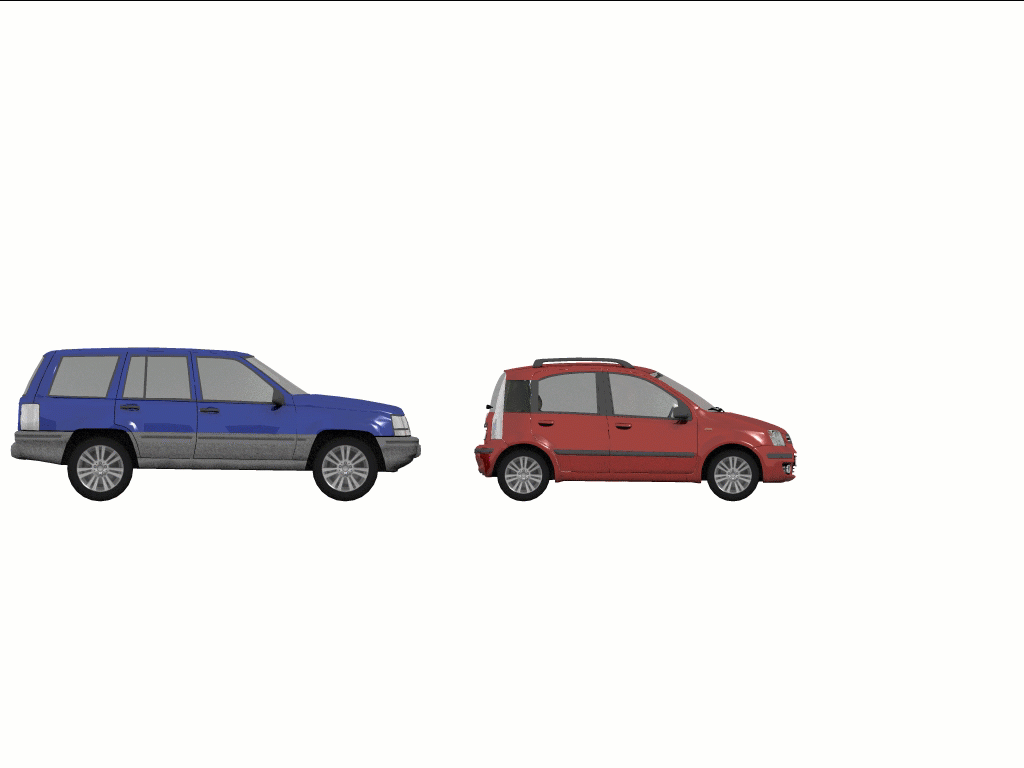
That is, in the case where each vehicle is equal in stiffness, the expected maximum crush on each vehicle is also equal. By default, Virtual CRASH places x-y position of the impulse centroid at the geometrial center of the overlapping bounding box volume whose length is given by \(C_{T}(t_{max})\), which is a reasonable first approximation. For example, in figure below, the red vehicle has a pre-impact speed of 30 mph (44 fps) and impacts the blue vehicle at rest on its driver side. The depth of penetration is 30 msec. Therefore, the first impulse exchange occurs after the red vehicle travels 44 fps x 0.03 secs = 1.32 feet beyond the position of first overlap. As explained in the User’s Guide (VC5 | VC4 | VC3), the reported deformation values simply indicate the distance between the bounding boxes and the impluse centroid position along the normal axis. In this configuration, the impulse vectors are aligned with the normal axis.
In the figure below we see a more complex situation, where the red vehicle is at a 45 degree angle with respect to the blue vehicle. The red vehicle is traveling 60 mph (88 fps) pre-impact. It, therefore, moves 2.64 feet into the blue vehicle before impulses are exchanged. Again, the impulse centroid is placed at the geometrical center of the overlap volume (shown in red). Note, the deformation reported in the left side control panel, in this case, is greater for the red vehicle than for the blue vehicle, despite the impulse centroid being at the geometrical center of the overlap region. Again, the reported deformation value here is simply the distance between the vehicle's rectangular bounding box and the impulse centroid along the normal axis. Since the red vehicle's bumper is rounded on the corners, the actual implied maximum crush damage (distance between the outer vehicle mesh polygons and the impulse centroid) is approximately the same as the blue vehicle's.
The user, of course, can also directly modify the placement of the impulse centroid within the crush volume as needed for the particular case. This is discussed in the User’s Guide (VC5 | VC4 | VC3). For example, one might want to position the impulse centroid such that the maximum damaged delivered to each vehicle is in accordance with equations (34) and (35). Below we see an example of moving the impulse centroid using the mouse by first disabling auto-position.
While a simple linear force model like Hooke’s Law is a mathematically convenient model to characterize a vehicle’s resistance to compressive loading, vehicles may exhibit variable stiffness as a function of region impacted, impact speed, or as a function of crush damage itself; therefore, while one may be justified in adjusting the relative placement of the impulse centroid to represent the effect of the relative vehicle stiffness, this isn’t necessarily a “tight” constraint that must be satisfied. One is also justified in treating the impulse centroid location as an optimization parameter which can be adjusted within reason and according to one’s own scientific or engineering judgment. For example, when performing a CRASH3 calculation for a t-bone impact with wheel involvement, it is customary to increase the side impact stiffness coefficient in the zone about the wheel to account for increased structural rigidity in that area. This generally has the effect of moving the force centroid position closer to the wheel. In Virtual CRASH, to account for wheel involvement, one can simply move the impulse centroid closer to the wheel. On the matter of impulse centroid placement, we quote Brach, who published his rigid body dynamics based collision model in 1977 (quote from section 6.5.2.2 of reference [5]):
"A residual crush surface of a vehicle is reached in a relatively short time, but still represents a change from the undeformed shape as a function of time and space. That is, it is a three-dimensional, dynamic event... [It is assumed] a common point exists that represents the point of application of the intervehicle impulse. [This point], often referred to as the impact center [or impulse centroid], is easy to define mathematically; it is the point of application of the resultant vector impulse. It represents the point of application of the intervehicle force averaged over space and time. Unfortunately, the location of the [the impulse centroid] is never is exactly known, and must be estimated. One approach is to lay out a plan view of the residual crush and use the centroid of the crushed area. Another is to use a point on the residual crush surface, because some springback of the body occurs. Another is to use the maximum crush surface [see SAE 940564]. Whatever method is used, judgment of the analysis is necessary."
From \(k\) to \(B\)
Using our 1-D spring model we can develop reasonable values to use for depth of penetration by examining the \(B\) coefficients of various types of vehicles. Recall, the assumption used by CRASH3, which was originally developed by Campbell [12, 13], is that the force response of a vehicle as a function of crush depth can be represented as the sum of an ensemble of infinitesimal linear springs imaged to run along the perimeter of the vehicle. For a permanent crush profile distributed along the width \(w\) of a vehicle, the crush profile can be described by the function \(C_{P}(w)\). We can then calculate the total spring force, generalized for a 2-dimensional array, by performing the integral:
$$F_{max} = \int^{W}_{0} dw’ \cdot (A + B\cdot C_{P}(w’)) $$
and the energy absorbed at the moment of maximum engagement is:
$$ E_{max} = {1 \over 2} \int^{W}_{0} dw' \cdot B \cdot \left({A \over B} + C_{P}(w') \right)^2$$

Here \(A\) and \(B\) are the usual “stiffness coefficients,” where \(A\) (units [Force]/[Length]) is typically understood as the “pre-load” force term, characterizing the force per unit width threshold for permanent deformation. \(B\) (units [Force]/[Area]) is understood as the generalized spring stiffness value characterizing the spring resistance to compression per unit width. Using staged collision data to characterize the vehicle stiffness constant value \(k\), \(B\) can be approximated by \(B = {k \over w}\), where \(W\) is the width of direct contact damage. Using this \(B\) along with knowledge of the no-damage closing-speed limit, \(A\) can be obtained. As was discussed above, this approximation of \(A\) and \(B\) assumes a homogenous stiffness response by the contact surface; that is, that both \(A\) and \(B\) are constant as a function of \(w\) and crush damage.
In the case of a single-value crush measurement, we arrive back at a 1-dimensional approximation, where the force simply becomes:
$$F_{max} = \left( A + B \cdot C_{P} \right) \cdot W $$
The linear force form of this equation is suggestive, where one may identify the product \(B \cdot W\) as the linear spring constant term \(k\), corresponding to the spring-stiffness value for dynamic deflection. Indeed, this interpretation is supported in prior work [14]. With this identification, we now have a way to associate the commonly derived \(B\) stiffness coefficient with \(k\) from above, and thus, can estimate reasonable values for depth of penetration based on \(B\) coefficients.
Typical \(\Delta t_{p}\) values
Using “generic" vehicle data, we can now examine typical \(B\) stiffness coefficient values and vehicle weights for various vehicle classes and derive corresponding \(t_{max}\) values, and from these, expected \(\Delta t_{p}\) values. The tables below show the weights and \(B\) coefficients for various vehicle classes from [15]. The uncertainties (standard deviations) on these values are also shown.
A ROOT monte carlo analysis script was written to test all pairwise combinations of these vehicle types to estimate the expected \(\Delta t_{p} \) values for all possible configurations: front to front, front to rear, front to side, rear to side [16]. These combinations assume full-width engagement, where the minimum width value was used for each pair tested, and the impacts are in-line. Here the width is simply twice the distance from CG to right side. The ROOT script used uniform probability density functions to test all width, weight, and \(B\) stiffness values ranging from the average value less one standard deviation to the average value plus one standard deviation. The resulting histogram is shown below.

From these results, our range of typical depth of penetration values is between 10 and 60 milliseconds. For infinitely rigid objects, the theoretical lower limit is of course 0 milliseconds. Note, these values assume full width engagement, but for offset collisions, the direct damage width will be lower, thereby decreasing the effective stiffness, and increasing depth of penetration time. Virtual CRASH allows the user to set this value to anything between 0 seconds to 60 milliseconds, but uses a default value of 30 milliseconds, which as demonstrated here is an excellent representative value for a large range of impact configurations between various vehicle types.
Non-central collisions
Accounting for non-central impacts simply requires using “effective mass” terms such that for vehicle \(i\) [8, 17]:
$$ m_{i} \rightarrow \gamma_{i} \cdot m_{i} $$
where
$$ \gamma_{i} = { k_{i}^2 \over k_{i}^2 + h_{i}^2 } $$
where \(h_{i}\) is the lever-arm and the radius of gyration is given by:
$$ k_{i}^2 = {I_{i} \over m_{i}}$$
The net effect of torque on our vehicle due to a non-zero lever-arm is then completely contained within the \(\gamma\) term. In the limit that the \(h_{i} \rightarrow \infty\), we have \(m_{i} \rightarrow 0 \). In the other extreme where \(h_{i} \rightarrow 0\) for an in-line impact, we have \(m_{i} \rightarrow m_{i} \). Since the effective mass terms can only be as large as the original masses, the reduced mass can only be reduced by non-central collisions. Therefore, the effect of non-central collision would be to reduce the depth of penetration time. We therefore see again, the range from 0 to 60 milliseconds is a reasonable one.
References
[1] Slibar A., “ Die mechanischen GmndsXtze des StoBvorganges freier und gefuhrter Korper und ihre Anwendung auf den StoBvorgang van Fabrzeugen.” Archiv for Unfallforschung, 2. Jg., H. 1, 1966, 31ff.
[5] See for example, the Planar Impact Mechanics Analysis software module of VCRWare by Brach Engineering (brachengineering.com), and the associated SAE Text: “Vehicle Accident Analysis and Reconstruction Methods”, R. Brach and R. Brach, SAE International, Warrendale, Pennsylvania, 2005.
[6] See for example, Day, T. and Hargens, L., “An Overview of the Way EDSMAC Computes Delta-V”, Paper No. 880069, SAE, Warrendale, PA.
[7] “CRASH3 User’s Guide and Technical Manual”, NHTSA, DOT Report HS 805 732, 1981.
[8] See page 2.20 of reference [7].
[9] Depth of penetration is introduced in the Virtual CRASH User’s Guide (VC5 | VC4 | VC3).
[10] See Chapter 2 of reference [7].
[12] Campbell, K., “Energy Basis for Collision Severity”, Paper No. 740565, SAE, Warrendale, PA.