< Appendix 2 | Contents | Appendix 4 >

Appendix 3 | The Virtual CRASH Coordinate System

Introduction

Virtual CRASH uses three coordinate systems to fully describe the conditions of a vehicle in motion. The vehicle is defined as a rigid body object that moves under the influences of external forces.

Earth Frame – The Fixed Global Coordinate System

Virtual CRASH uses a right-handed coordinate system in which $z$-axis is aligned anti-parallel with gravitational acceleration. Note, this is a different convention than SAE in which the $z$-axis points parallel with gravity. The vehicle center-of-gravity is location specified within a fixed inertial reference (Earth) frame by its $(x,y,z)$ coordinate (see below).

Vehicle Position

Each vehicle has its own local frame of reference. Starting with the vehicle at rest on the ground $(x-y)$ plane at $(0, 0, z_{cg})$, let us define the $\hat{x}'$ axis as the unit vector extending from the vehicle center-of-gravity, parallel with the x-y plane, directed to point through the front-end, mid-way between the driver and passenger side (see below). Let us define the $\hat{y}'$ axis as the unit-vector orthogonal to the $\hat{x}'$ axis, parallel to the x-y plane, extending from the center-of-gravity directed to point through the driver side. Finally, let $\hat{z}' = \hat{x}' \times \hat{y}'$.

Vehicle Orientation

Transformations from Earth Frame to Vehicle Frame

In Virtual CRASH, vehicle dynamics is simulated in three-dimensions, and therefore requires mathematical representation of vehicle orientations. Vehicle orientations are most conveniently described procedurally, in terms of each the local Vehicle Frame’s orientation with respect to the Earth frame. Starting with a vehicle aligned with the Earth Frame, any arbitrary orientation can be defined with three rotations, applied in order:

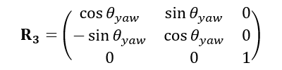
(1) First, we apply the yaw rotation. In this case, the yaw rotation transformation matrix taking a vector from Earth Frame to Vehicle Frame is given by:

We can find the yaw angle for a vehicle arbitrarily oriented by projecting the local $\hat{x}'$ axis onto the x-y plane. This is given by: $\bar{x}'_{xy} = \hat{x}' - (\hat{x}' \cdot \hat{z}) \cdot \hat{z}$. The vehicle yaw angle is given by the angle between $\bar{x}'_{xy}$ and $\hat{x}$, which is given by: $\frac{\bar{x}'_{xy}}{|\bar{x}'_{xy}|} \cdot \hat{x} = \cos \theta_{yaw}$.

(2) Second, we apply the pitch rotation about the rotated $\hat{y}'$ axis. The pitch rotation transformation matrix taking a vector from Earth Frame to Vehicle Frame is given by:

The pitch angle is given by the angle between the $\hat{x}'$ axis and $\bar{x}'_{xy}$. This is defined by the solution to: $\frac{\bar{x}'_{xy}}{|\bar{x}'_{xy}|} \cdot \hat{x}' = \cos \theta_{pitch}$, where the rotations occur about the axis given by $\hat{x}' \times \bar{x}'_{xy}$.

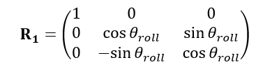
(3) Finally, we apply the roll angle. The roll rotation transformation matrix taking a vector from Earth Frame to Vehicle Frame is given by:

Therefore, after first setting $\theta_{yaw}$ and $\theta_{pitch}$, $\hat{y}'$ is taken to a new rotated configuration away from its initial pre-rotated configuration $\hat{y}_i'$. Let us now rotate the vehicle about the local $\hat{x}'$ axis such that $\hat{y}' \rightarrow \hat{y}'^*$. The roll angle is given by the solution to: $\hat{y}' \cdot \hat{y}'^* = \cos \theta_{roll}$.

The total transformation matrix $\mathbf{T}$, that takes a vector from Earth Frame to Vehicle Frame, is therefore given by the matrix product:

Tire Orientation

Each tire has its own orientation within the local vehicle frame. Let us define the direction of the $j$th wheel’s heading by the $\hat{x}_j$ axis. The wheel slip angle $\alpha_j$ is given by the angle between the velocity at the wheel hub, $\bar{v}_j$, and the wheel’s heading $\hat{x}_j$. The steering angle, $\varphi_j$, is given by the angle between the wheel’s heading $\hat{x}_j$ and the local frame $\hat{x}'$ axis.

< Appendix 2 | Contents | Appendix 4 >