

Chapter 27 | The Smart Optimizer
Introduction
With the Winter 2025 Software Update, Virtual CRASH 6 introduces the new Smart Optimizer, an advanced search and optimization tool designed to streamline the accident reconstruction process. This powerful system automatically iterates over your selected input variables, such as speeds, positions, impact parameters, and more, in order to rapidly generate a range of simulation scenarios that align with the physical evidence. By intelligently evaluating each iteration against your defined constraints and objectives, the Smart Optimizer identifies the combinations that most accurately satisfy your reconstruction goals. Whether you are refining initial conditions, testing alternative hypotheses, or exploring the sensitivity of specific parameters, the Smart Optimizer significantly reduces the time required to arrive at defensible and evidence-based solutions. Read on to learn more about how this amazing feature, available only in Virtual CRASH 6, can enhance both the speed and precision of your simulation workflow!
A Gentle Introduction | Slide-to-Stop Analysis
To begin using the Smart Optimizer, simply create your simulation model as you normally would. You can model an initial hypothesis, or you can leave all simulated objects at rest. In this example, we are evaluating the pre-braking speed of a red vehicle (see below) based on a known braking distance. The driver applied the brakes after striking a pedestrian. Of course, this trivial “slide-to-stop” analysis can be performed manually by using the real-time feedback in Virtual CRASH and quickly scanning across v(t=0) in the Dynamics menu, or by using the V0 fast-control icon. For this first example illustrating the Smart Optimizer, we will allow it to automatically iterate over a user-specified range of possible pre-braking speeds to see whether it can correctly converge on the known 50 mph initial speed.
Once your simulation scenario is set up with all necessary objects in place, you will need to insert “Position / Orientation Constraint” objects into your scene if your intention is to satisfy any position, orientation, or speed constraints. Left-click on Optimizer > Position / Orientation Constraint to activate constraint object mode.
Next, select your time-step of interest either by using the time slider or by left-clicking directly on an interposition for the unfrozen object to which you want to add constraint objects. In this example, we will hover over the red subject vehicle. The object will highlight in light blue to confirm it is ready for selection. Hold+left-click and drag away from the object to create a constraint object associated with that parent. You can add as many constraint objects as needed, scrubbing forward and backward in time while in constraint object creation mode. Constraint objects can also be cloned in “use copy” mode. Note that it is not necessary to use the time slider when placing constraint objects, but you may find it convenient, because if your parent object is in motion, the constraint object will be placed near the region and orientation of interest corresponding to your selected time-step.
Right-click to exit constraint object adding mode. In this simple example, we are only using one constraint object, placed at the documented rest position of our vehicle.
In [F2] or [F3] mouse cursor control mode, you can adjust the constraint object’s position and orientation as needed. This can also be done in the position-local and rotation-local menus.
Next, open the “misc” menu to set the various tolerances for the constraint object. In this case, we will set “radius” to 0.5 ft, “delta yaw” to 2 degrees, “min v” to 0 mph, and “max v” to 0.5 mph. The Smart Optimizer will attempt to find the user-enabled simulation inputs that produce outputs falling within these tolerance ranges. How these input values are used, and how valid outputs are identified, is described in more detail below.
Next, to access the Smart Optimizer, left-click Optimizer > Show Optimizer from the menu bar. You can also open the Smart Optimizer by left-clicking the Smart Optimizer button on the upper toolbar, or by pressing the graph button on the lower toolbar.
Once the graph window opens, adjust its size as needed so you can clearly read the left-side panel. Make sure “optimizer” is highlighted in the upper-left corner of the graph window rather than “controllers” or “diagrams”.
Next, locate the rigid body objects of interest in the list on the left-side of the graph window. In our example, we want the Smart Optimizer to solve for the initial speed that allows the vehicle to traverse the known braking distance. Therefore, we will activate Vehicle 1 > dynamics > v (t=0s) by left-clicking on the empty box to the right of its name. Once clicked, a check mark appears, confirming that this parameter is now active. Notice that the hierarchy mirrors the standard menu structure found in the left-side control panel for all rigid body objects. Note, the known braking distance is implied by the initial position of the vehicle and the rest position indicated by the inserted constraint object (with target speed range < 0.5 mph).
After a parameter is enabled, you can set its lower limit (“min value”) and upper limit (“max value”) in the “parameter settings” menu under Properties. These values define the range the Smart Optimizer is permitted to use when selecting input values for the enabled parameter. If possible, try to set a reasonable but narrow min/max range to speed up the optimization process. Reasonable ranges can often be estimated from hand calculations, data from literature, experience, preliminary simulation analyses, etc.
To re-access the parameter menu later, simply left-click directly on the parameter’s name in the hierarchy.
In this simple use case, we will have the Smart Optimizer test initial speeds from 0 to 100 mph and an initial yaw angle within ±5 degrees, in case the initial yaw angle is suboptimal given the known rest position. For any enabled optimization parameter, the “relative” toggle can be enabled. When enabled, the “value” input field will be automatically populated with the corresponding value from the parent object’s input field, which can be considered a best or reasonable estimate. A search window can then be defined above and below this estimate using the “delta value” input field.
In our example, the red vehicle was set up in the 3D environment with rotation-local yaw = −32.864 degrees based on the lane configuration in the 3D environment, and therefore this is the reasonable first estimate. When rotation-local is enabled in the optimizer window, this initial yaw value is automatically populated in the “value” input field. Note that at the time of the initial release, the “value” field will not update automatically if the user changes the initial state of the parent object after “relative” is enabled.
Finally, open the "optimizer" menu under "properties". In this menu, you will see both the inputs and outputs associated with the Smart Optimizer. By default, the long-time classic optimization approach using a genetic algorithm is selected (1). This algorithm begins by creating an initial population of trial simulations (Generation 0), each with inputs randomly distributed across the user-specified parameter ranges. Every trial is evaluated against the constraints, and the population is sorted by total deviation. The algorithm then selects parent-simulations from among the best performers and creates child-simulations by combining information from those parents while allowing some additional variation of input values. These children compete with their parents, the population is re-sorted, and the process repeats across successive generations. The search continues until either a solution falls within the specified tolerances (max deviation) or the maximum number of generations is reached. If "exit after max. number of generations" is enabled, the best simulation found is returned, and its enabled inputs are automatically programmed into the corresponding input fields. If this option is disabled (the default state), the process starts over with new random seeds. The general process is illustrated below.
Note the default parameter set described below works well in many cases, but these settings can be modified depending on the specific use case.
Genetic Algorithm
The genetic algorithm inputs are as follows:
Size of Population: The number of candidate simulations (iterations) maintained in each generation. Larger populations provide greater initial diversity across the input data space but increase computational cost per generation.
Max. Number of Generations: The absolute stopping criterion: the maximum number of generations the Smart Optimizer will run before terminating if “exit after max. generations” is enabled; otherwise, optimizer will reset with new random seed and continue running.
Transfer Ratio: The fraction of simulations that is preserved unchanged between generations. These are the best performing simulations (best “fitness”) that survive directly into the next generation without modification to input data.
Mutate Probability: The probability that a child-simulation will have random variations added to all its input data after it's created. When triggered, mutation perturbs every parameter simultaneously.
Crossover Probability: The probability that a child-simulation is created by blending two parent-simulations versus being a direct copy of one parent-simulation. If crossover triggers: child-simulation input parameters are sampled uniformly between the two parent values. If crossover doesn't trigger: child-simulation inputs are an exact copy of one parent (before mutation).
Once you have set the parameters in the optimizer menu, verify that physics is not paused (the gears icon should not be highlighted). Then left-click the play button in the graph window to activate the Smart Optimizer.
As the Smart Optimizer runs, you will see a real-time visualization of the current trial in the 3D environment. By default, only a subset of trials will be displayed within the 3D environment. Pressing the play button at the bottom of the screen (next to the teapot icon) will display all iterations as the Smart Optimizer runs.
You will also see real-time results on the left side of the graph window in the “optimizer” section. For each iteration performed by the solver, the total deviation is computed as the weighted RMS deviation of the individual deviation terms enabled by the user.
$$ \text{minimize: } f_i(\alpha_{1,i}, \alpha_{2,i}, \ldots, \alpha_{M,i}) = \frac{1}{\sqrt{\tilde{N}}} \sqrt{\sum_{j=1}^{N} w_j \cdot \left( \frac{\tilde{p}_{j,i} - p_{j,\text{target}}}{p_{j,\text{norm}}} \right)^2} $$
where:
\(M\) = number of enabled input parameters specified within min/max range
\(N\) = number of constraints
\(\alpha\) = automatically varied input parameter
\(i\) = optimization "trial simulation" index
\(j\) = optimization parameter constraint index
\(w_j\) = weight for constraint parameter \(j\)
\(\tilde{p}_{j,i}\) = parameter \(j\) OUTPUT value for trial simulation \(i\)
\(p_{j,\text{target}}\) = parameter \(j\) TARGET constraint value (for example, \(\Delta\text{yaw} = 0°\))
\(p_{j,\text{norm}}\) = normalization factor to unitless terms which can be summed
\(\tilde{N} = \sum_{j=1}^{N} w_j\)
For each position/orientation constraint object created for a given parent, Virtual CRASH evaluates all time-steps during each optimization iteration to identify the time-step that yields the minimum distance to the constraint object. This process is illustrated below for trial simulation \(i\), where the displacement vector from the constraint object to the vehicle position is computed at each integration time-step. Each displacement vector is indexed by time-step number (here the time-step size is exaggerated for illustration purposes). For this trial simulation, the position, orientation, and speed values are sampled from time-step 5 to evaluate the corresponding deviation for trial \(i\).
This process is repeated for all constraint objects in the scene. Virtual CRASH then computes the individual deviation terms for each enabled parameter for each constraint object. These are listed below:
Position Deviation: For a given constraint object, the position deviation is computed using the displacement vector between the constraint object and the parent object's position at the nearest interposition (time-step) within the current optimization iteration. This displacement vector is then normalized by the distance normalization factor, which is given by the displacement vector from initial position to nearest interposition to constraint object. The magnitude of the normalized deviation vector is then squared and multiplied by the “position weight” input value (default 100%). If the user-defined “radius” tolerance is greater than zero, the deviation displacement magnitude is first reduced by the radius. If this difference is less than or equal to zero (i.e., the deviation lies within the tolerance circle), the position deviation for that constraint object is set to 0 for the optimization iteration.
Orientation Deviation: For a given constraint object, the yaw orientation deviation is computed using the absolute difference in yaw (|delta yaw|) between the constraint object and the parent object at the nearest interposition (time-step). This value is normalized by the angle normalization factor, which is defined as 180 degrees. The normalized deviation is squared and multiplied by the “orientation weight” input value (default 100%). Note, at the time of the initial release, yaw angles are bounded between -180 to +180 degrees. If the user-defined “delta yaw” tolerance is greater than zero, the computed |delta yaw| is reduced by this tolerance. If this difference is less than zero (i.e., within tolerance), the orientation deviation for that constraint object is set to 0 for the optimization iteration. Note: The orientation deviation term can be disabled by unchecking the “use orientation” toggle.
Speed Deviation: For a given constraint object, the speed deviation is computed using the nearest interposition (time-step) speed of the parent object. If this speed is less than or equal to the user-defined “min v”, the deviation is taken relative to min v. If the speed is greater than or equal to the user-defined “max v”, the deviation is taken relative to max v. This speed difference is then normalized by the speed normalization factor (100 kph), squared, and multiplied by the “velocity weight” input value (default 100%). If the nearest time-step speed lies between min v and max v (inclusive), the speed deviation for that constraint object is set to 0 for the optimization iteration. Note: The velocity deviation term can be disabled by unchecking the “use velocity” toggle.
There are also constraints available through ees (impulse) objects. These will be discussed further below.
Delta v (impulse/mass) Deviation: This can be enabled in the optimizer window by using the checkbox for the desired ees object (cumulative delta v via dynamics info will come in a future update). This must be a user contact. For each optimization iteration, if delta v for the selected ees object is less than or equal to the user-defined "min value", the deviation is taken relative to the min value. If the delta v is greater than or equal to the user-defined "max value", the deviation is taken relative to the max value. This delta v difference is then normalized by the speed normalization factor (100 kph), squared, and multiplied by the "weight" input value (default 100%). If delta v lies between the min value and max value (inclusive), the speed deviation for that constraint is set to 0 for the optimization iteration. Note: the min/max values and weight are input in the optimizer window > properties > constraint menu. The procedure described here is the same for “ees”, “v pre-impact”, and “v post-impact” deviation terms, all of which can also be enabled in the optimizer window.
Deformation Deviation: This can be enabled in the optimizer window by using the checkbox for the desired ees object. This must be a user contact. For each optimization iteration, if deformation for the selected ees object is less than or equal to the user-defined "min value", the deviation is taken relative to the min value. If the deformation is greater than or equal to the user-defined "max value", the deviation is taken relative to the max value. This deformation difference is then normalized by 1 meter, squared, and multiplied by the "weight" input value (default 100%). If deformation lies between the min value and max value (inclusive), the deformation deviation for that constraint is set to 0 for the optimization iteration. Note: the min/max values and weight are input in the optimizer window > properties > constraint menu.
Impulse pdof (local, sae) Deviation: This can be enabled in the optimizer window by using the checkbox for the desired ees object. This must be a user contact. For each optimization iteration, if pdof for the selected ees object is less than or equal to the user-defined "min value", the deviation is taken relative to the min value. If the pdof is greater than or equal to the user-defined "max value", the deviation is taken relative to the max value. This pdof difference is then normalized by angle normalization factor (180 degrees), squared, and multiplied by the "weight" input value (default 100%). If pdof lies between the min value and max value (inclusive), the pdof deviation for that constraint is set to 0 for the optimization iteration. Note: the min/max values and weight are input in the optimizer window > properties > constraint menu.
All individual deviation terms are combined using a weighted RMS, and the final result is returned and displayed in the “iteration deviation” output field in the “optimizer” menu. The minimum deviation over all iterations in the current population is shown in the “deviation” output field.
The matrix here shows deviation terms for the vehicle, representing the individual terms inside the radical of the deviation function (see equation 1). Each column corresponds to a constraint object in the scene, and each row corresponds to an enabled constraint type (position, orientation, speed). A separate table for constraints related to impulse exchanges is also shown (disabled in this case). The values shown are the squared, normalized, weighted deviations for each term before they are summed and passed through the square root.
In this example, all terms are equally weighted at 100%, though each term can have its own unique linear weight factor set in the constraint object's "misc" menu.
If a constraint value falls within the user-defined tolerance (radius for position, delta yaw for orientation, or between min v and max v for speed), the corresponding deviation term is set to zero for that constraint object. This allows you to define acceptable tolerance windows based on the uncertainty in your physical evidence.
Note that a single vehicle can have as many constraint objects as needed, with each constraint object placed at a different location in the 3D environment. As you add more objects to your simulation with additional constraints and constraint terms enabled, this matrix will grow to include more terms in the deviation function summation. The Smart Optimizer ultimately seeks the simulation that minimizes the weighted RMS of all terms.
As the Smart Optimizer runs, you will see a graph on the right that displays the iteration deviation as a function of iteration within the population. These values are represented by blue vertical bars (dark blue if from the prior generation and light blue if from the current generation). If an iteration deviation is less than 5%, its bar will appear light orange. Population members whose iteration deviation falls below the user-defined “max. deviation” exit condition will be shown in green. The lowest deviation for all iterations within the current generation will be shown in the upper right corner.
Once at least one iteration returns a deviation below the user-specified maximum deviation, the Smart Optimizer will complete the remaining iterations for the current generation and then terminate. If no such iteration is found, the Smart Optimizer will continue running until it reaches the maximum number of generations or until the pause or stop buttons are pressed.
Once the Smart Optimizer has finished, you can left-click on any enabled parameter in the left-side hierarchy to view its output distribution for the final generation. The parameter values will be graphed as a function of iteration, sorted from least to greatest deviation.
In the results shown below, we improved our solution by requiring the maximum deviation to be no greater than 0.01% before terminating the optimization process. Doing so, of course, increases the total run-time of the Smart Optimizer. Again, any iterations remaining in the final generation with deviation less than or equal to 0.01% will be shown in green. In our case, only 1 iteration out of 40 in the final generation had its deviation less than 0.01%, and therefore the Smart Optimizer stopped.
You can hover over the vertical bar graphics in the graph to refresh the ghosted visualizations that show the nearest simulated positions to each constraint object for the iteration corresponding to the bar under the mouse cursor. This provides a quick understanding of the variation in position and orientation among the iterations in the final generation. You can also left-click any vertical bar in the graph to load the corresponding simulation input values and update the 3D environment to display that specific scenario.
By left-clicking on any disabled parameter name in the hierarchy, the right-side graph will switch to display the iteration error for the final generation. As before, you can hover over the graph bars to view the ghosted vehicle representations relative to the constraint objects, or you can left-click on a bar to load its corresponding input data directly into the simulation.
Below we see a similar analysis where we allow rotation-local yaw to vary ±45 degrees. On the left is the deviation vs. yaw and speed landscape; on the right, the resulting deviation as a function of iteration. With each generation, the elite population drifts toward lower deviation values as better combinations of initial yaw and speed are tested.
Below on the left, we see the envelope of elite speeds after each generation. The narrowing envelope converges to the true value over only a few generations. On the right, we see the deviation for each iteration. Over successive generations, the best results converge to the minimum of the deviation function at the true speed (50 mph).
The workflow in the slide-to-stop example above is reviewed in the video below.
Assessing Simulation Sensitivity
We will now expand the range of adhesion values for our vehicle in order to explore the effect of drag factor uncertainty. To illustrate the concept, we will suppose our adhesion value is in the range from 0.7 to 0.8 and examine how this broader range widens the initial speed range for our solution. We are using a deliberately wide uncertainty window here to make the idea clear. For this study, we have disabled optimization of the initial yaw and instead hold it fixed at the best value obtained from the prior run.
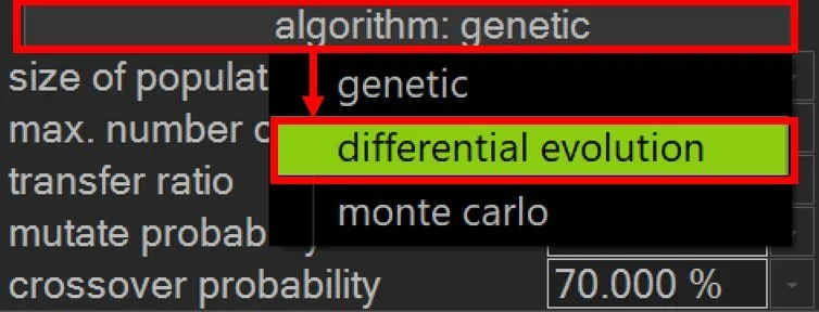
For this task, we will use differential evolution.
Differential evolution is another evolutionary algorithm that often outperforms a genetic algorithm on continuous, numerical problems because its mutation step uses the difference between existing solutions to guide the search more efficiently (2). While a genetic algorithm typically relies on random perturbations that resemble taking random steps in the search space, differential evolution uses vector-based operations to produce a more informed and directed step. Both approaches then use crossover to blend information from the newly generated candidate with the current best solution, followed by a selection process that retains the superior option for the next generation. Use the algorithm drop down to select “differential evolution”.
You’ll find new input parameters, defined below:
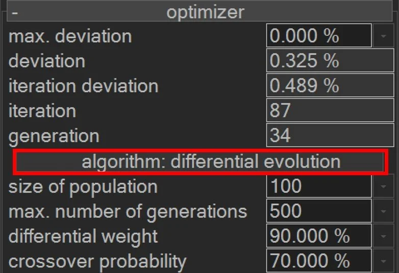
Differential Weight: The scaling factor that controls how strongly the difference between two randomly selected candidate simulations influences the creation of a new candidate. Higher differential weight values produce larger steps across the input space, which increases exploration and helps the Smart Optimizer search widely. Lower values produce smaller, more conservative steps that focus on refining promising regions of the search space. Note: the option “monte carlo” is the same algorithm as differential evolution, but with differential weight = 0.
Crossover Probability: The probability that each input value in the new candidate simulation will be taken from the mutated vector rather than from the existing parent simulation. High crossover probabilities promote stronger mixing of candidate solutions and encourage the Smart Optimizer to move decisively toward new variations created through mutation. Lower probabilities preserve more of the original parent values, which can stabilize the search but may limit the rate of improvement.
Differential evolution can provide better performance than a genetic algorithm for our constrained, continuous search across the two-dimensional parameter space in this example. It can potentially explore a complex, continuous solution space more efficiently and more consistently.
Our strategy in this example is to lower the “max. deviation limit” input value so that the Smart Optimizer is required to run through many generations before it can meet the constraint. We will then simply observe the Smart Optimizer’s progress and stop the process manually once all candidates in a given generation fall below 1% deviation.
For our optimizer constraint object, we set both the min v and max v to 0, and we set the radius to 0. Tight constraints, in addition to the minimum possible “max. deviation limit” practically ensure no stopping condition will be satisfied, and so we can run the Smart Optimizer until all iterations within a generation are filled with deviation less than 1%. Below we see the final distribution of deviation values after a few minutes of running.
Next, we examine the distribution of adhesion values across the population to verify that the full range of possible values is represented. As expected, the distribution spans the complete range.
Finally, we determine the minimum and maximum initial speeds that satisfy the slide-to-stop distance requirement implied by our constraint object and the vehicle’s initial position (107.1 ft stopping distance). The resulting range of 47–51 mph matches the interval predicted by hand calculations for a vehicle braking from 50 mph on a flat, level surface.
This illustrates how the Smart Optimizer can be used to evaluate a simulation’s sensitivity to its input parameters and to identify feasible parameter ranges under multi-dimensional constraints. Although we focused on adhesion-driven variation in initial speed in this simple scenario, the same methodology extends naturally to a broad set of input parameters for far more complex simulations.
Collision Analysis
The Smart Optimizer can be a big time saver for collision analysis since the input parameter space tends to span numerous dimensions, which are prohibitive to scan via manual multi-dimensional grid searching. Below we show a collision analysis setup based on RICSAC Test 3. The vehicles' initial positions are at the moment of contact. Constraint objects are set for each vehicle at their documented rest positions. An intermediate constraint object is used for Vehicle 2 since its post-impact trajectory follows an arcing path. Note, intermediate constraint objects should have "use velocity" disabled without specific data to suggest a likely range at the given location. In this study, our objective is to find the pre-impact speed for Vehicle 1 that results in simulated outcomes consistent with our vehicle position and orientation constraints.
Here, the Smart Optimizer is enabled. The minimum parameter set for this analysis is selected, with reasonable initial minimum and maximum values set for each parameter. In order to scan across potential effect points of contact, a user contact EES object was created with contact > "auto-position" disabled. Once auto-position is disabled, the user contact EES object position can be added to the optimization parameter list. Since the position-local y value of the EES object is of particular importance in this case to generate post-impact yaw rate needed to redirect Vehicle 1, only position-local y was added to the parameter list. Restitution can be particularly important, and therefore the user contact's restitution value was also included. Induced steer is added to Vehicle 2. Thus we are searching for a deviation function global minimum within a 4-dimensional volume. In this case, we'll use the default settings for the genetic algorithm, but use a strict exit condition of "max. deviation" = 0.2%.
The matrix below shows deviation terms for both vehicles (see equation 1). In this example, all terms are equally weighted. Vehicle 2 has two constraint objects in the scene (one at the mid-point of the post-impact trajectory and one at rest) and each contributes to the weighted RMS calculation. See the slide-to-stop example above for a detailed explanation of how deviation terms are computed.
When optimizing over many parameters, you may find it useful to adjust min/max values as it becomes clear what the narrower range should be. Be careful not to bias your results in doing so since there may be unique and non-intuitive combinations of input parameters that satisfy your constraints. Here, it quickly becomes clear that the possible range for Vehicle 2's induced steering angle must be quite low for it to follow the arcing trajectory indicated by the evidence. By shrinking the volume of the search space, you can more quickly arrive at an optimal solution.
After a few minutes, we exit out of the Smart Optimizer with the best pre-impact speed estimate of 20.5 mph (within 1 mph of the true value).
A video of this optimization is shown below (playback sped up).
Impulse-based constraints
It is also possible to add optimization parameters based on impulse exchanges. Below, we see the user contact impulse has under "Object 1" and "Object 2" options to include deviation terms based on EES, delta-v (impulse / mass), v pre-impact, v post-impact, deformation, and impulse PDOF (local, SAE). Any parameter shown highlighted in red can be added as an optimization constraint.
In our example, we'll remove the rest position constraint of Vehicle 1 and see if instead the Smart Optimizer can obtain a best estimate of pre-impact speed if we include a delta-v constraint. Here we'll use 8.9 mph. Below we see the updated matrix of deviation terms for this analysis.
After re-running the optimization, the optimal speed value is again found to be 20.5 mph.
Pedestrian Impact Analysis
Constraint objects can also be added for multibodies. Simply left-click on Optimizer > Position/Orientation Constraint, then left-click on your unfrozen multibody in your scene and position the constraint object as needed. In the example shown below, we use two constraint objects. One for an intermediate position near ground contact and the second for the rest position. Of course, for the intermediate position, the "use velocity" toggle should be disabled. Using two such constraint objects can help ensure the multibody travels from impact to rest along a straight vector, reducing trajectories that scatter laterally and then tumble back to the rest constraint object. Note, the pose of the optimizer object only indicates the initial pose of the multibody. The rest pose of your simulated multibody is in no way used by the Smart Optimizer.
The matrix here shows deviation terms for each object in the simulation (see equation 1). In this example, all terms are equally weighted, though each can have its own unique weight factor. Note that in the initial release, multibodies do not have an orientation constraint option, so "n/a" appears in the table. Additionally, since pedestrian impacts are modeled using "default-auto" impulse exchanges, there are no possible impulse-related constraints. See the slide-to-stop example for a detailed explanation of deviation term calculations.
In our example here, the final solution from the Smart Optimizer is consistent with our expectations from Searle.
A video of this optimization is shown below (playback sped up).
Bicycle/Motorcycle Accident Analysis
In the example below, we attempt to solve for the bullet SUV pre-impact speed that leads to the rest positions of the bicycle, rider, and SUV. Note, as of the initial release, only the yaw angle of the constraint objects is configurable. Therefore, only the yaw angle of the bicycle will be added to the deviation function if "use orientation" is enabled.
Below we see the final optimized solution.
The matrix below shows deviation terms for each object in the simulation (see equation 1). In this example, all terms are equally weighted, though each can have its own unique weight factor. Note that in the initial release, multibodies do not have an orientation constraint option, so "n/a" appears in the table. See the slide-to-stop example for a detailed explanation of deviation term calculations.
A video of this optimization is shown below (playback sped up).
In the example below, we have a motorcycle T-bone crash based on WREX 2000 CT8. A constraint object was set at the rest position and orientation of each vehicle. Here, a user contact was created in order to iterate over impulse centroid locations.
The matrix below shows deviation terms for each object in the simulation (see equation 1). In this example, all terms are equally weighted.
Here the Smart Optimizer stops on a result within a few percent the true motorcycle pre-impact speed.
A video of this optimization is shown below (playback sped up).
Trajectory and Sequence Analysis
The Smart Optimizer can also be used for programming sequences. In the example below, we use three constraint objects to guide our simulated vehicle around the right turn. The final two constraint objects help to ensure the vehicle's final trajectory is straight and follows the lane. Our simulated vehicle is programmed with the minimum number of sequences required to complete the desired action (always a good practice).
The time values for sequences 2 and 3 and the target steering angle were solved for by the Smart Optimizer.
The matrix below shows deviation terms for the vehicle (see equation 1). In this example, all terms are equally weighted. Note that a single vehicle can have as many constraint objects as needed, with corresponding constraint objects placed in the 3D environment. See the slide-to-stop example for additional details on deviation calculations.
A video of this optimization is shown below (playback sped up).
Tractor-Trailer Reversing
In the example below, the Smart Optimizer is used to synchronize the sensitive interplay between steering and timing to reverse the tractor-trailer into a warehouse loading bay. Three sequences are the minimum number needed to execute this action. The Smart Optimizer also solves for sequence 3's pedal position to bring the system to rest at the proper location. Two constraint objects are used, both for the trailer only, to guide it in a straight line to the loading bay. In keeping with the recommendations below, no constraints on the tractor's speed, position, or orientation are used since they are already correlated with the trailer's parameters.
The matrix below shows deviation terms for the trailer (see equation 1). In this example, all terms are equally weighted. Note that a single vehicle can have as many constraint objects as needed, with corresponding constraint objects placed in the 3D environment. See the slide-to-stop example for additional details on deviation calculations.
Here we see the final optimizer solution.
A video of this optimization is shown below (playback sped up).
General Recommendations when using the Smart Optimizer
Build your simulation with your best hypothesis as you normally would, then allow the Smart Optimizer to iterate from that starting point. Set your objects at best-estimate initial positions, orientations, speeds, and sequences. Then enable the Smart Optimizer to scan across critical parameters where you have reasonable uncertainty. As you enable search parameters in the optimizer window, consider enabling "relative" mode in the "parameter" menu. This uses the current value from your initial simulation and automatically populates the "value" field using your current input, saving setup time. Note: before enabling "relative" mode, ensure the Smart Optimizer is paused and your initial values are set as intended. If the optimizer is running when you enable "relative," it will capture the current trial value rather than your intended baseline. You can toggle "relative" off and on again to re-read the current value from the simulation input field.
Be conservative with enabled search parameters. More is not always better. The more parameters (or dimensions) you enable for the Smart Optimizer to scan through, the larger the search volume within which the global minimum deviation sits. While enabling additional parameters gives the optimizer more flexibility to find solutions that match physical evidence, it may also substantially increase the size of the search space. This means the algorithm may require significantly more time, and potentially more generations, to converge on an optimal solution. Start with the parameters you're most uncertain about, and only add additional dimensions if the optimizer struggles to achieve acceptable deviation values.
Be conservative with constraints. As the Smart Optimizer runs, it tests candidate simulations by calculating deviation terms for each constraint you enable. There is an effective “tug-of-war” as various deviation terms within equation (1) compete to be individually minimized within the summation. When constraints pull in conflicting directions, the optimizer must find compromise solutions that may not fully satisfy any single constraint. Fewer constraints allow for a smoother deviation function landscape, which can speed up convergence and produce clearer results. Start by running the optimization using only the most important constraints, then add additional constraints as needed to satisfy your requirements. This incremental approach also helps you understand which constraints are driving the solution and whether any are conflicting with one another.
Work incrementally. Consider focusing on one vehicle at a time, disabling search parameters and constraint objects for other vehicles. You can run the Smart Optimizer as many times as needed within your project to solve for any combination of inputs.
Guide the optimizer toward candidate solutions. You can “squeeze” your search parameters as the Smart Optimizer runs to guide it toward potential solutions. While the optimization is running, left-click on the enabled parameter names to see the performance graph for that parameter. If it is clear the Smart Optimizer is converging toward a particular range of values for a given parameter, adjust that parameter's "value" and "delta value" (if relative mode is enabled) or "min value" and "max value" (if relative mode is disabled) to focus the search within more useful regions of the search space. This will speed up the optimization process. For example, if you are programming a left turn maneuver, you might set the minimum steering angle to 0 degrees since you know the vehicle will not be steering to the right during this phase. Similarly, if physical evidence indicates a vehicle was traveling between 40 and 60 mph, there is no need to allow the optimizer to search speeds outside that range. However, do not get too aggressive with squeezing ranges as you do not want to bias your results or inadvertently exclude valid solutions. After adjusting the range of your values, press the "play" button again to restart the Smart Optimizer with the new limits. This technique is also useful if you see the optimizer has become stuck in a local minimum rather than finding the global minimum for the deviation function. By adjusting the parameter ranges, you effectively give the algorithm a fresh start within a more targeted search region, which can help it escape suboptimal solutions.
Take advantage of constraint tolerances and weights. For example, if you know a pedestrian came to rest within an area in your scene with an uncertainty of 3 feet, you can indicate that in the multibody constraint object's "radius" input field in the "misc" menu. This allows the optimizer to treat any solution landing within that radius as equally valid, helping the Smart Optimizer converge more quickly to low deviation solutions. If guiding the bullet vehicle to its final rest position is more critical than the pedestrian's, you can indicate that by setting the pedestrian's "position weight" term to a value lower than 100% in the "misc" menu. This tells the optimizer to prioritize matching the vehicle's rest position over the pedestrian's when the two goals compete. You can make these changes on the fly while the optimizer runs to see how such adjustments guide the optimizer toward more acceptable solutions.
Consider increasing your population size. If your objective is to perform a sensitivity analysis, where you want a large list of candidate simulations that all satisfy your max deviation requirement, then increase the "size of population" input field in the "optimizer" menu. Enable "apply to all" to ensure that all simulations in the final population satisfy your "max deviation" requirement. Once the Smart Optimizer finishes, left-click on each enabled search parameter to see the min/max range within the graph window. You can also scrub across the graph itself to understand the variability of the solutions by watching the trajectories update in your 3D environment. This gives you a visual sense of the range of physically plausible scenarios that fit your evidence constraints.
Run multiple times from different starting points. If you suspect the optimizer may be finding local minima, try running it again with different initial conditions or parameter ranges. Consistent results across multiple runs increase confidence that you have found a robust solution.
Save your work. Before starting a long optimization run, save your project file. Consider saving multiple instances of your project file as you work, especially after the optimizer finds promising solutions. This protects against losing progress and gives you the ability to return to earlier states if you want to explore different optimization scenarios.
Document your settings. When you find a solution that works, make note of which parameters you enabled, what ranges you used, and which constraints were active. This may help you as your case evolves and requires additional simulation work.
Minimize time-max if possible. The larger time-max is, the longer each iteration will take since each trial simulation must run from 0 to time-max. If possible, set time-max only as long as needed to calculate all relevant deviation terms. After the Smart Optimizer finishes, you can always increase time-max as needed for your final visualization.
Optimize for speed. Whatever generally slows down a manual simulation analysis will also slow the Smart Optimizer: complex 3D terrain meshes with high polygon counts, systems with joint couplings, small integration time-step sizes, and so on. Use the same approaches you already rely on for speeding up iteration cycle times to help the Smart Optimizer run as quickly as possible.
Notes:
(1) There are many publicly available resources explaining how genetic algorithms work. One such reference is: Whitley, D. (1994). "A Genetic Algorithm Tutorial." Statistics and Computing, 4(2), 65-85 (download). The Smart Optimizer uses a proprietary implementation based on genetic algorithm principles.
(2) There are many publicly available resources explaining how the differential evolution algorithm works. One such reference is: Storn, R. & Price, K. (1997). "Differential Evolution – A Simple and Efficient Heuristic for Global Optimization over Continuous Spaces." Journal of Global Optimization, 11(4), 341-359 (download). The Smart Optimizer applies a proprietary version of this algorithm. The Smart Optimizer uses a proprietary implementation based on differential evolution principles.
© 2025 Virtual CRASH, LLC. All Rights Reserved